FAQ

What is VictoriaMetrics Anomaly Detection (vmanomaly)? #

VictoriaMetrics Anomaly Detection, also known as vmanomaly, is a service for detecting unexpected changes in time series data. Utilizing machine learning models, it computes and pushes back an “anomaly score” for user-specified metrics. This hands-off approach to anomaly detection reduces the need for manual alert setup and can adapt to various metrics, improving your observability experience.

Please refer to our QuickStart section to find out more.

Note: vmanomaly is a part of enterprise package. You need to get a free trial license for evaluation.

What is anomaly score? #

Among the metrics produced by vmanomaly (as detailed in vmanomaly output metrics), anomaly_score is a pivotal one. It is a continuous score > 0, calculated in such a way that scores ranging from 0.0 to 1.0 usually represent normal data, while scores exceeding 1.0 are typically classified as anomalous. However, it’s important to note that the threshold for anomaly detection can be customized in the alert configuration settings.

The decision to set the changepoint at 1.0 is made to ensure consistency across various models and alerting configurations, such that a score above 1.0 consistently signifies an anomaly, thus, alerting rules are maintained more easily.

Note: anomaly_score is a metric itself, which preserves all labels found in input data and (optionally) appends custom labels, specified in writer - follow the link for detailed output example.

How is anomaly score calculated? #

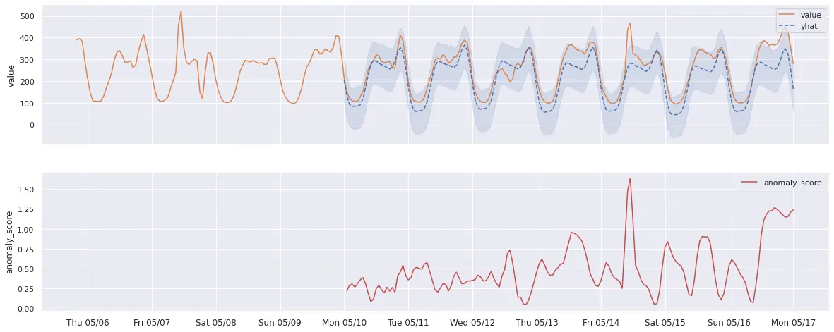
For most of the univariate models that can generate yhat, yhat_lower, and yhat_upper time series in their output (such as Prophet or Z-score), the anomaly score is calculated as follows:

If yhat (expected series behavior) equals y (actual value observed), then the anomaly score is 0.
If y (actual value observed) falls within the [yhat_lower, yhat_upper] confidence interval, the anomaly score will gradually approach 1, the closer y is to the boundary.
If y (actual value observed) strictly exceeds the [yhat_lower, yhat_upper] interval, the anomaly score will be greater than 1, increasing as the margin between the actual value and the expected range grows.

Please see example graph illustrating this logic below:

p.s. please note that additional post-processing logic might be applied to produced anomaly scores, if common arguments like min_dev_from_expected or detection_direction are enabled for a particular model. Follow the links above for the explanations.

How does vmanomaly work? #

vmanomaly applies built-in (or custom) anomaly detection algorithms, specified in a config file.

All the models generate a metric called anomaly_score
All produced anomaly scores are unified in a way that values lower than 1.0 mean “likely normal”, while values over 1.0 mean “likely anomalous”
Simple rules for alerting: start with anomaly_score{“key”=”value”} > 1
Models are retrained continuously, based on schedulers section in a config, so that threshold=1.0 remains actual
Produced scores are stored back to VictoriaMetrics TSDB and can be used for various observability tasks (alerting, visualization, debugging).

What data does vmanomaly operate on? #

vmanomaly operates on data fetched from VictoriaMetrics, where you can leverage full power of MetricsQL for data selection, sampling, and processing. Users can also apply global filters for more targeted data analysis, enhancing scope limitation and tenant visibility.

Respective config is defined in a reader section.

Handling noisy input data #

vmanomaly operates on data fetched from VictoriaMetrics using MetricsQL queries, so the initial data quality can be fine-tuned with aggregation, grouping, and filtering to reduce noise and improve anomaly detection accuracy.

Output produced by vmanomaly #

vmanomaly models generate metrics like anomaly_score, yhat, yhat_lower, yhat_upper, and y. These metrics provide a comprehensive view of the detected anomalies. The service also produces health check metrics for monitoring its performance.

Choosing the right model for vmanomaly #

Selecting the best model for vmanomaly depends on the data’s nature and the types of anomalies to detect. For instance, Z-score is suitable for data without trends or seasonality, while more complex patterns might require models like Prophet.

Also, starting from v1.12.0 it’s possible to auto-tune the most important params of selected model class, find the details here.

Please refer to respective blogpost on anomaly types and alerting heuristics for more details.

Still not 100% sure what to use? We are here to help.

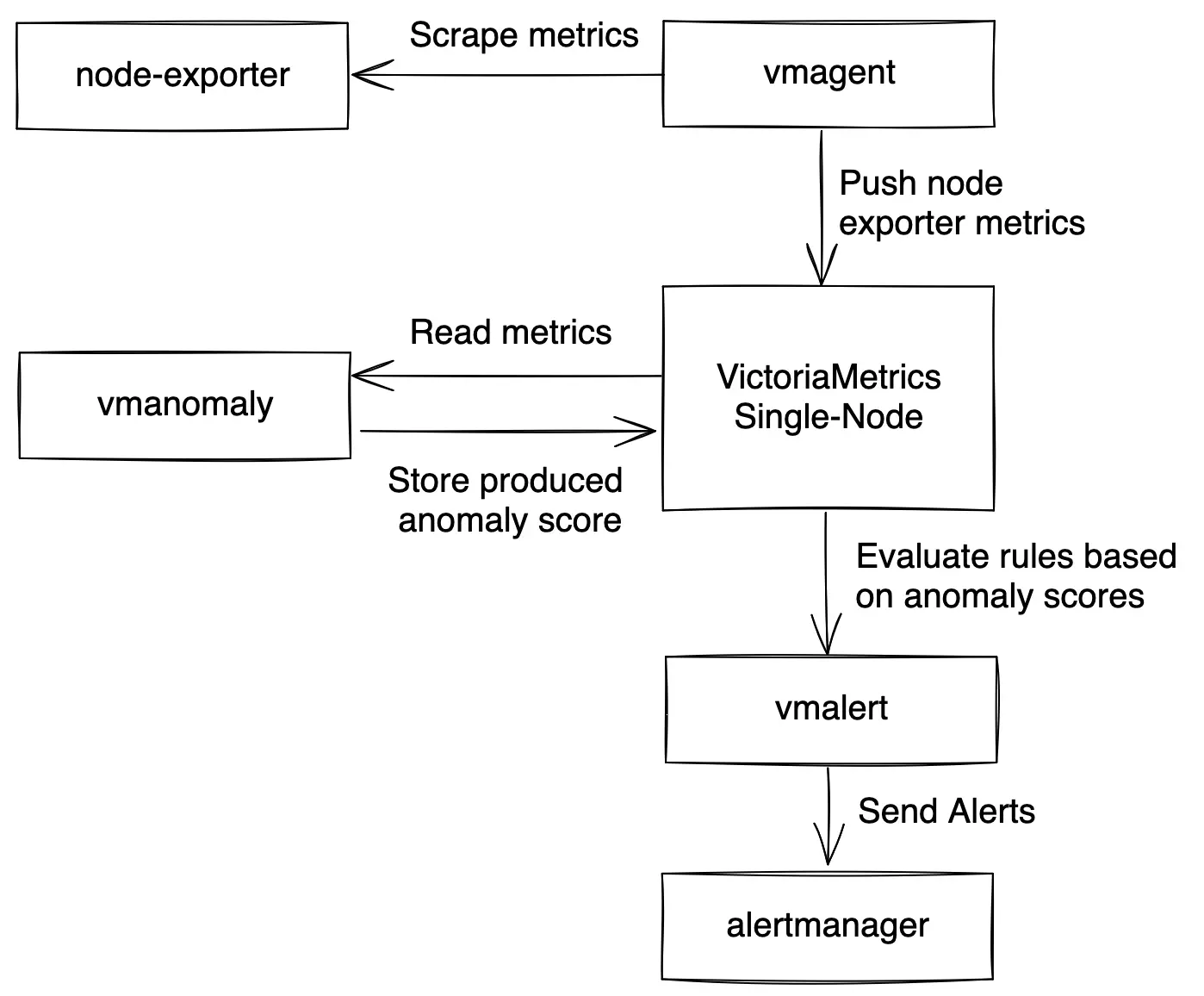
Alert generation in vmanomaly #

While vmanomaly detects anomalies and produces scores, it does not directly generate alerts. The anomaly scores are written back to VictoriaMetrics, where an external alerting tool, like vmalert, can be used to create alerts based on these scores for integrating it with your alerting management system.

Preventing alert fatigue #

Produced anomaly scores are designed in such a way that values from 0.0 to 1.0 indicate non-anomalous data, while a value greater than 1.0 is generally classified as an anomaly. However, there are no perfect models for anomaly detection, that’s why reasonable defaults expressions like anomaly_score > 1 may not work 100% of the time. However, anomaly scores, produced by vmanomaly are written back as metrics to VictoriaMetrics, where tools like vmalert can use MetricsQL expressions to fine-tune alerting thresholds and conditions, balancing between avoiding false negatives and reducing false positives.

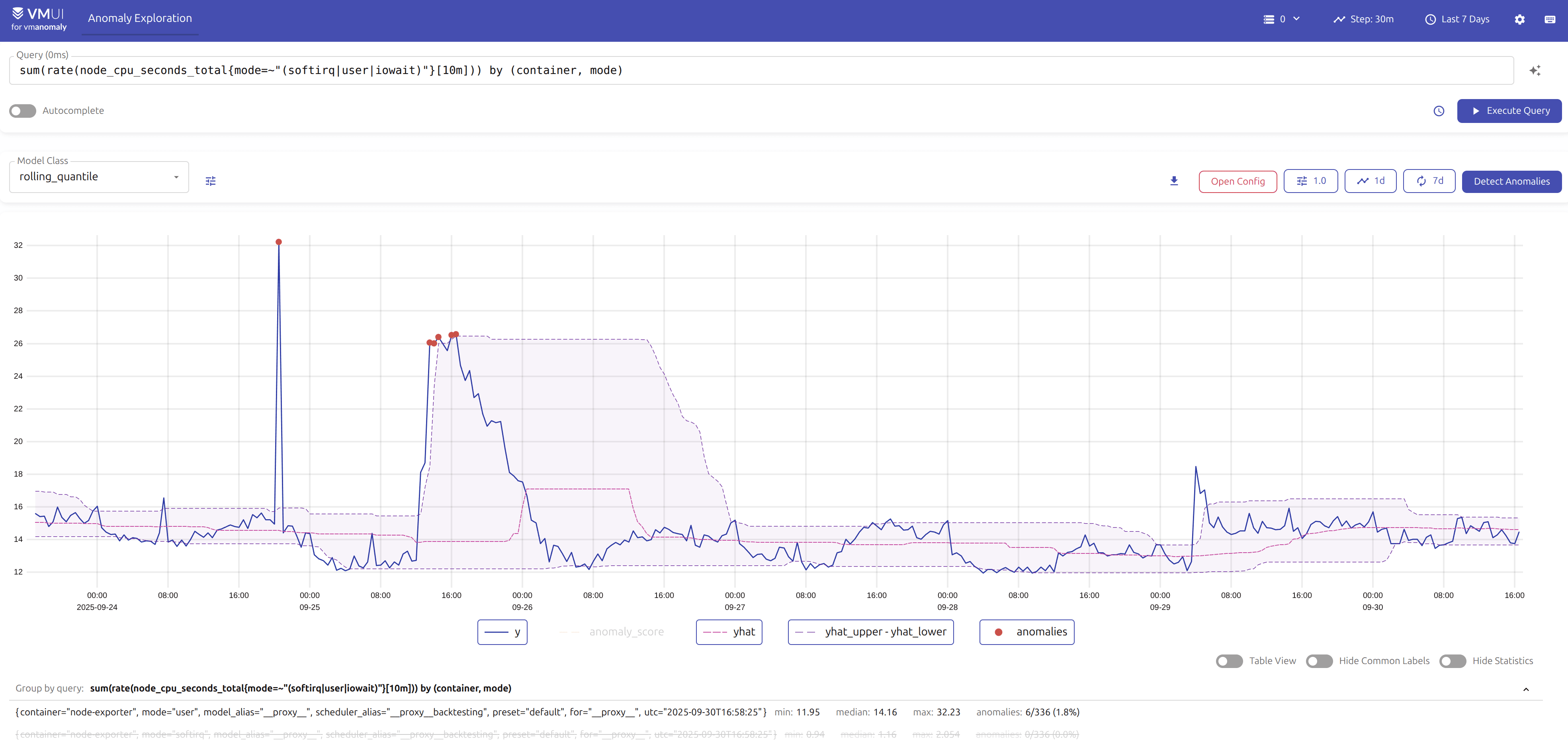
How to backtest particular configuration on historical data? #

Starting from v1.7.2 you can produce (and write back to VictoriaMetrics TSDB) anomaly scores for historical (backtesting) period, using BacktestingScheduler component to imitate consecutive “production runs” of PeriodicScheduler component. Please find an example config below:

schedulers:
  scheduler_alias:
    class: 'backtesting' # or "scheduler.backtesting.BacktestingScheduler" until v1.13.0
    # define historical period to backtest on
    # should be bigger than at least (fit_window + fit_every) time range
    from_iso: '2024-01-01T00:00:00Z'
    to_iso: '2024-01-15T00:00:00Z'
    # copy these from your PeriodicScheduler args
    fit_window: 'P14D'
    fit_every: 'PT1H'
    # number of parallel jobs to run. Default is 1, each job is a separate OneOffScheduler fit/inference run.
    n_jobs: 1

models:
  model_alias1:
    # ...
    schedulers: ['scheduler_alias']  # if omitted, all the defined schedulers will be attached
    queries: ['query_alias1']  # if omitted, all the defined queries will be attached
    # https://docs.victoriametrics.com/anomaly-detection/components/models/#provide-series
    provide_series: ['anomaly_score']  
  # ... other models

reader:
  datasource_url: 'some_url_to_read_data_from'
  queries:
    query_alias1: 'some_metricsql_query'
  sampling_frequency: '1m'  # change to whatever you need in data granularity
  # other params if needed
  # https://docs.victoriametrics.com/anomaly-detection/components/reader/#vm-reader

writer:
  datasource_url: 'some_url_to_write_produced_data_to'
  # other params if needed
  # https://docs.victoriametrics.com/anomaly-detection/components/writer/#vm-writer

# optional monitoring section if needed
# https://docs.victoriametrics.com/anomaly-detection/components/monitoring/

Configuration above will produce N intervals of full length (fit_window=14d + fit_every=1h) until to_iso timestamp is reached to run N consecutive fit calls to train models; Then these models will be used to produce M = [fit_every / sampling_frequency] infer datapoints for fit_every range at the end of each such interval, imitating M consecutive calls of infer_every in PeriodicScheduler config. These datapoints then will be written back to VictoriaMetrics TSDB, defined in writer section for further visualization (i.e. in VMUI or Grafana)

Resource consumption of vmanomaly #

vmanomaly itself is a lightweight service, resource usage is primarily dependent on scheduling (how often and on what data to fit/infer your models), # and size of timeseries returned by your queries, and the complexity of the employed models. Its resource usage is directly related to these factors, making it adaptable to various operational scales. Various optimizations are available to balance between RAM usage, processing speed, and model capacity. These options are described in the sections below.

On-disk mode #

Note: Starting from v1.13.0, there is an option to save anomaly detection models to the host filesystem after the fit stage (instead of keeping them in memory by default). This is particularly useful for resource-intensive setups (e.g., many models, many metrics, or larger fit_window argument) and for 3rd-party models that store fit data (such as ProphetModel or HoltWinters). This reduces RAM consumption significantly, though at the cost of slightly slower infer stages. To enable this, set the environment variable VMANOMALY_MODEL_DUMPS_DIR to the desired location. If using Helm charts, starting from chart version 1.3.0 .persistentVolume.enabled should be set to true in values.yaml.

Note: Starting from v1.16.0, a similar optimization is available for data read from VictoriaMetrics TSDB. To use this, set the environment variable VMANOMALY_DATA_DUMPS_DIR to the desired location.

Here’s an example of how to set it up in docker-compose using volumes:

services:
  # ...
  vmanomaly:
    container_name: vmanomaly
    image: victoriametrics/vmanomaly:v1.17.2
    # ...
    ports:
      - "8490:8490"
    restart: always
    volumes:
      - ./vmanomaly_config.yml:/config.yaml
      - ./vmanomaly_license:/license
      # map the host directory to the container directory
      - vmanomaly_model_dump_dir:/vmanomaly/tmp/models
      - vmanomaly_data_dump_dir:/vmanomaly/tmp/data
    environment:
      # set the environment variable for the model dump directory
      - VMANOMALY_MODEL_DUMPS_DIR=/vmanomaly/tmp/models/
      - VMANOMALY_DATA_DUMPS_DIR=/vmanomaly/tmp/data/
    platform: "linux/amd64"
    command:
      - "/config.yaml"
      - "--licenseFile=/license"

volumes:
  # ...
  vmanomaly_model_dump_dir: {}
  vmanomaly_data_dump_dir: {}

For Helm chart users, refer to the persistentVolume section in the values.yaml file. Ensure that the boolean flags dumpModels and dumpData are set as needed (both are enabled by default).

Online models #

Note: Starting from v1.15.0 with the introduction of online models, you can additionally reduce resource consumption (e.g., flatten fit stage peaks by querying less data from VictoriaMetrics at once).

Reduced Latency: Online models update incrementally, which can lead to faster response times for anomaly detection since the model continuously adapts to new data without waiting for a batch fit.
Scalability: Handling smaller data chunks at a time reduces memory and computational overhead, making it easier to scale the anomaly detection system.
Improved Resource Utilization: By spreading the computational load over time and reducing peak demands, online models make more efficient use of system resources, potentially lowering operational costs.

Here’s an example of how we can switch from (offline) Z-score model to Online Z-score model:

schedulers:
  periodic:
    class: 'periodic'
    fit_every: '1h'
    fit_window: '2d'
    infer_every: '1m'
  # other schedulers ...
models:
  zscore_example:
    class: 'zscore'
    schedulers: ['periodic']
    # other model params ...
# other config sections ...

to something like

schedulers:
  periodic:
    class: 'periodic'
    fit_every: '180d'  # we need only initial fit to start
    fit_window: '4h'  # reduced window, especially if the data doesn't have strong seasonality
    infer_every: '1m'  # the model will be updated during each infer call
  # other schedulers ...
models:
  zscore_example:
    class: 'zscore_online'
    min_n_samples_seen: 120  # i.e. minimal relevant seasonality or (initial) fit_window / sampling_frequency
    schedulers: ['periodic']
    # other model params ...
# other config sections ...

As a result, switching from the offline Z-score model to the Online Z-score model results in significant data volume reduction, i.e. over one week:

Old Configuration:

fit_window: 2 days
fit_every: 1 hour

New Configuration:

fit_window: 4 hours
fit_every: 180 days ( >1 week)

The old configuration would perform 168 (hours in a week) fit calls, each using 2 days (48 hours) of data, totaling 168 * 48 = 8064 hours of data for each timeseries returned.

The new configuration performs only 1 fit call in 180 days, using 4 hours of data initially, totaling 4 hours of data, which is magnitudes smaller.

P.s. infer data volume will remain the same for both models, so it does not affect the overall calculations.

Data Volume Reduction:

Old: 8064 hours/week (fit) + 168 hours/week (infer)
New: 4 hours/week (fit) + 168 hours/week (infer)

Handling large queries in vmanomaly #

If you’re dealing with a large query in the queries argument of VmReader (especially when running within a scheduler using a long fit_window), you may encounter issues such as query timeouts (due to the search.maxQueryDuration server limit) or rejections (if the search.maxPointsPerTimeseries server limit is exceeded).

We recommend upgrading to v1.17.2, which introduced the max_points_per_query argument (both global and query-specific) for the VmReader. This argument overrides how search.maxPointsPerTimeseries flag handling (introduced in v1.14.1) is used in vmanomaly for splitting long fit_window queries into smaller sub-intervals. This helps users avoid hitting the search.maxQueryDuration limit for individual queries by distributing initial query across multiple subquery requests with minimal overhead.

By splitting long fit_window queries into smaller sub-intervals, this helps avoid hitting the search.maxQueryDuration limit, distributing the load across multiple subquery requests with minimal overhead. To resolve the issue, reduce max_points_per_query to a value lower than search.maxPointsPerTimeseries until the problem is gone:

reader:
  # other reader args
  max_points_per_query: 10000  # reader-level constraint
  queries:
    sum_alerts:
      expr: 'sum(ALERTS{alertstate=~'(pending|firing)'}) by (alertstate)'
      max_points_per_query: 5000  # query-level override
models:
    prophet:
      # other model args
      queries: [
        'sum_alerts',
      ]
# other config sections

Alternative workaround for older versions #

If upgrading is not an option, you can partially address the issue by splitting your large query into smaller ones using appropriate label filters:

For example, such query

reader:
  # other reader args
  queries:
    sum_alerts:
      expr: 'sum(ALERTS{alertstate=~'(pending|firing)'}) by (alertstate)'
models:
    prophet:
      # other model args
      queries: [
        'sum_alerts',
      ]
# other config sections

can be modified to:

reader:
  # other reader args
  queries:
    sum_alerts_pending:
      expr: 'sum(ALERTS{alertstate='pending'}) by ()'
    sum_alerts_firing:
      expr: 'sum(ALERTS{alertstate='firing'}) by ()'
models:
    prophet:
      # other model args
      queries: [
        'sum_alerts_pending',
        'sum_alerts_firing',
      ]
# other config sections

Please note that this approach may not fully resolve the issue if subqueries are not evenly distributed in terms of returned timeseries. Additionally, this workaround is not suitable for queries used in multivariate models (especially when using the groupby argument).

Scaling vmanomaly #

Note: As of latest release we do not support cluster or auto-scaled version yet (though, it’s in our roadmap for - better backends, more parallelization, etc.), so proposed workarounds should be addressed manually.

vmanomaly can be scaled horizontally by launching multiple independent instances, each with its own MetricsQL queries and configurations:

By splitting queries, defined in reader section and spawn separate service around it. Also in case you have only 1 query returning huge amount of timeseries, you can further split it by applying MetricsQL filters, i.e. using “extra_filters” param in reader. See the example below.
or models (in case you decide to run several models for each timeseries received i.e. for averaging anomaly scores in your alerting rules of vmalert or using a vote approach to reduce false positives) - see queries arg in model config
or schedulers (in case you want the same models to be trained under several schedules) - see schedulers arg model section and scheduler component itself

Here’s an example of how to split on extra_filters, based on extra_filters reader’s arg:

# config file #1, for 1st vmanomaly instance
# ...
reader:
  # ...
  queries:
    extra_big_query: metricsql_expression_returning_too_many_timeseries
    extra_filters:
      # suppose you have a label `region` with values to deterministically define such subsets
      - '{region="region_name_1"}'
      # ...

# config file #2, for 2nd vmanomaly instance
# ...
reader:
  # ...
  queries:
    extra_big_query: metricsql_expression_returning_too_many_timeseries
    extra_filters:
      # suppose you have a label `region` with values to deterministically define such subsets
      - '{region="region_name_2"}'
      # ...

FAQ #