Data model #
What is a metric #
Simply put, metric is a numeric measure or observation of something.
The most common use-cases for metrics are:
- check how the system behaves at the particular time period;
- correlate behavior changes to other measurements;
- observe or forecast trends;
- trigger events (alerts) if the metric exceeds a threshold.
Structure of a metric #
Let’s start with an example. To track how many requests our application serves, we’ll define a metric with the
name requests_total.
You can be more specific here by saying requests_success_total (for only successful requests)
or request_errors_total (for requests which failed). Choosing a metric name is very important and supposed to clarify
what is actually measured to every person who reads it, just like variable names in programming.
Labels #
Every metric can contain additional meta-information in the form of label-value pairs:
      requests_total{path="/", code="200"}
requests_total{path="/", code="403"}
The meta-information - a set of labels in curly braces - gives us a context for which path and with what code
the request was served. Label-value pairs are always of a string type. VictoriaMetrics data model is schemaless,
which means there is no need to define metric names or their labels in advance. The user is free to add or change ingested
metrics anytime.
Actually, the metric name is also a label with a special name __name__.
The __name__ key could be omitted
Available from v1.111.0
for simplicity. So the following series are identical:
      requests_total{path="/", code="200"}
{__name__="requests_total", path="/", code="200"}
{"requests_total", path="/", code="200"}
Labels can be automatically attached to the time series written via vmagent or Prometheus . VictoriaMetrics supports enforcing of label filters for query API to emulate data isolation. However, the real data isolation can be achieved via multi-tenancy .
Time series #
A combination of a metric name and its labels defines a time series. For example,
requests_total{path="/", code="200"} and requests_total{path="/", code="403"}
are two different time series because they have different values for code label.
The number of unique time series has an impact on database resource usage. See what is an active time series and what is high churn rate docs for details.
Cardinality #
The number of unique
time series
is named cardinality. Too big number of unique time series is named high cardinality.
High cardinality may result in increased resource usage at VictoriaMetrics.
See
these docs
for more details.
Raw samples #
Every unique time series may consist of an arbitrary number of (value, timestamp) data points (aka raw samples) sorted by timestamp.
VictoriaMetrics stores all the values as float64
with extra compression
applied.
This allows storing precise integer values with up to 12 decimal digits and any floating-point values with up to 12 significant decimal digits.
If the value has more than 12 significant decimal digits, then the less significant digits can be lost when storing them in VictoriaMetrics.
The timestamp is a Unix timestamp
with millisecond precision.
Below is an example of a single raw sample in Prometheus text exposition format :
requests_total{path="/", code="200"} 123 4567890
- The
requests_total{path="/", code="200"}identifies the associated time series for the given sample. - The
123is a sample value. - The
4567890is an optional timestamp for the sample. If it is missing, then the current timestamp is used when storing the sample in VictoriaMetrics.
Time series resolution #
Resolution is the minimum interval between raw samples of the time series . Consider the following example:
      ----------------------------------------------------------------------
|              <time series>                 | <value> | <timestamp> |
| requests_total{path="/health", code="200"} |    1    |  1676297640 |
| requests_total{path="/health", code="200"} |    2    |  1676297670 |
| requests_total{path="/health", code="200"} |    3    |  1676297700 |
| requests_total{path="/health", code="200"} |    4    |  1676297730 |
....
Here we have a time series requests_total{path="/health", code="200"} which has a value update each 30s.
This means, its resolution is also a 30s.
In terms of
pull model
, resolution is equal
to scrape_interval and is controlled by the monitoring system (server).
For
push model
, resolution is an interval between
samples timestamps and is controlled by a client (metrics collector).
Try to keep time series resolution consistent, since some MetricsQL functions may expect it to be so.
Types of metrics #
Internally, VictoriaMetrics does not have the notion of a metric type. The concept of a metric type exists specifically to help users to understand how the metric was measured. There are 4 common metric types.
Counter #
Counter is a metric, which counts some events. Its value increases or stays the same over time.
It cannot decrease in general case. The only exception is e.g. counter reset,
when the metric resets to zero. The counter reset can occur when the service, which exposes the counter, restarts.
So, the counter metric shows the number of observed events since the service start.
In programming, counter is a variable that you increment each time something happens.
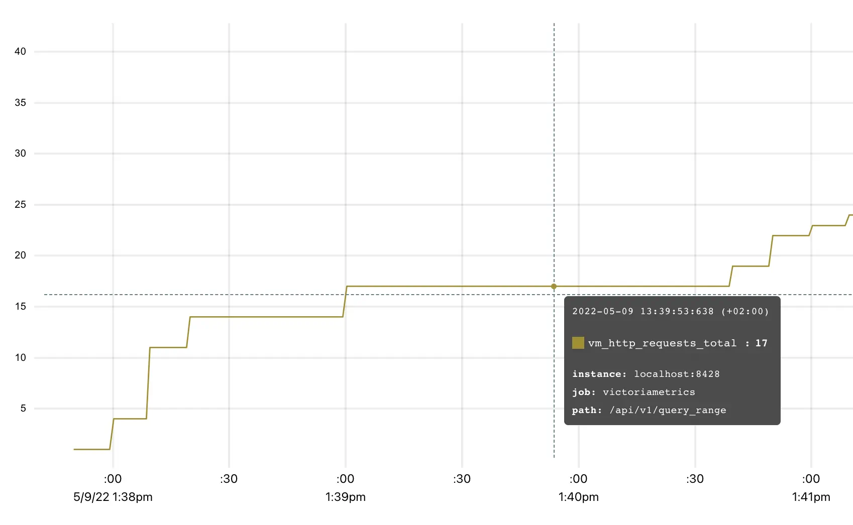
vm_http_requests_total is a typical example of a counter. The interpretation of a graph
above is that time series vm_http_requests_total{instance="localhost:8428", job="victoriametrics", path="api/v1/query_range"}
was rapidly changing from 1:38 pm to 1:39 pm, then there were no changes until 1:41 pm.
Counter is used for measuring the number of events, like the number of requests, errors, logs, messages, etc. The most common MetricsQL functions used with counters are:
- rate
- calculates the average per-second speed of metric change.
For example,
rate(requests_total)shows how many requests are served per second on average; - increase
- calculates the growth of a metric on the given
time period specified in square brackets.
For example,
increase(requests_total[1h])shows the number of requests served over the last hour.
It is OK to have fractional counters. For example, request_duration_seconds_sum counter may sum the durations of all the requests.
Every duration may have a fractional value in seconds, e.g. 0.5 of a second. So the cumulative sum of all the request durations
may be fractional too.
It is recommended to put _total, _sum or _count suffix to counter metric names, so such metrics can be easily differentiated
by humans from other metric types.
Gauge #
Gauge is used for measuring a value that can go up and down:
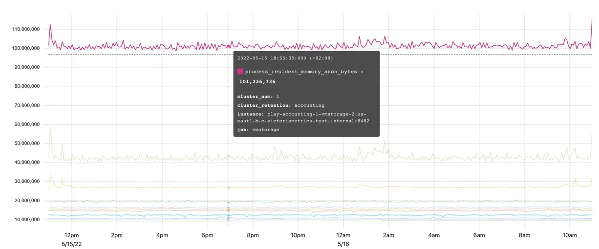
The metric process_resident_memory_anon_bytes on the graph shows the memory usage of the application at every given time.
It is changing frequently, going up and down showing how the process allocates and frees the memory.
In programming, gauge is a variable to which you set a specific value as it changes.
Gauge is used in the following scenarios:
- measuring temperature, memory usage, disk usage etc;
- storing the state of some process. For example, gauge
config_reloaded_successfulcan be set to1if everything is good, and to0if configuration failed to reload; - storing the timestamp when the event happened. For example,
config_last_reload_success_timestamp_secondscan store the timestamp of the last successful configuration reload.
The most common MetricsQL functions used with gauges are aggregation functions and rollup functions .
Histogram #
Histogram is a set of
counter
metrics with different vmrange or le labels.
The vmrange or le labels define measurement boundaries of a particular bucket.
When the observed measurement hits a particular bucket, then the corresponding counter is incremented.
Histogram buckets usually have _bucket suffix in their names.
For example, VictoriaMetrics tracks the distribution of rows processed per query with the vm_rows_read_per_query histogram.
The exposition format for this histogram has the following form:
      vm_rows_read_per_query_bucket{vmrange="4.084e+02...4.642e+02"} 2
vm_rows_read_per_query_bucket{vmrange="5.275e+02...5.995e+02"} 1
vm_rows_read_per_query_bucket{vmrange="8.799e+02...1.000e+03"} 1
vm_rows_read_per_query_bucket{vmrange="1.468e+03...1.668e+03"} 3
vm_rows_read_per_query_bucket{vmrange="1.896e+03...2.154e+03"} 4
vm_rows_read_per_query_sum 15582
vm_rows_read_per_query_count 11
The vm_rows_read_per_query_bucket{vmrange="4.084e+02...4.642e+02"} 2 line means
that there were 2 queries with the number of rows in the range (408.4 - 464.2]
since the last VictoriaMetrics start.
The counters ending with _bucket suffix allow estimating arbitrary percentile
for the observed measurement with the help of
histogram_quantile
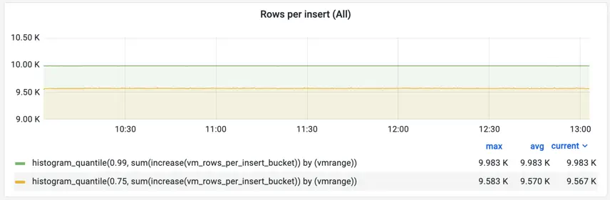
function. For example, the following query returns the estimated 99th percentile
on the number of rows read per each query during the last hour (see 1h in square brackets):
histogram_quantile(0.99, sum(increase(vm_rows_read_per_query_bucket[1h])) by (vmrange))
This query works in the following way:
- The
increase(vm_rows_read_per_query_bucket[1h])calculates per-bucket per-instance number of events over the last hour. - The
sum(...) by (vmrange)calculates per-bucket events by summing per-instance buckets with the samevmrangevalues. - The
histogram_quantile(0.99, ...)calculates 99th percentile overvmrangebuckets returned at step 2.
Histogram metric type exposes two additional counters ending with _sum and _count suffixes:
the
vm_rows_read_per_query_sumis a sum of all the observed measurements, e.g. the sum of rows served by all the queries since the last VictoriaMetrics start.the
vm_rows_read_per_query_countis the total number of observed events, e.g. the total number of observed queries since the last VictoriaMetrics start.
These counters allow calculating the average measurement value on a particular lookbehind window.
For example, the following query calculates the average number of rows read per query
during the last 5 minutes (see 5m in square brackets):
increase(vm_rows_read_per_query_sum[5m]) / increase(vm_rows_read_per_query_count[5m])
The vm_rows_read_per_query histogram may be used in Go application in the following way
by using the github.com/VictoriaMetrics/metrics
package:
      // define the histogram
rowsReadPerQuery := metrics.NewHistogram(`vm_rows_read_per_query`)

// use the histogram during processing
for _, query := range queries {
    rowsReadPerQuery.Update(float64(len(query.Rows)))
}
Now let’s see what happens each time when rowsReadPerQuery.Update is called:
- counter
vm_rows_read_per_query_sumis incremented by value oflen(query.Rows)expression; - counter
vm_rows_read_per_query_countincrements by 1; - counter
vm_rows_read_per_query_bucketgets incremented only if observed value is within the range (bucket) defined invmrange.
Such a combination of counter metrics allows
plotting Heatmaps in Grafana
and calculating quantiles
:
Grafana doesn’t understand buckets with vmrange labels, so the
prometheus_buckets
function must be used for converting buckets with vmrange labels to buckets with le labels before building heatmaps in Grafana.
Histograms are usually used for measuring the distribution of latency, sizes of elements (batch size, for example) etc. There are two implementations of a histogram supported by VictoriaMetrics:
- Prometheus histogram
. The canonical histogram implementation is
supported by most of
the client libraries for metrics instrumentation
. Prometheus
histogram requires a user to define ranges (
buckets) statically. - VictoriaMetrics histogram supported by VictoriaMetrics/metrics instrumentation library. Victoriametrics histogram automatically handles bucket boundaries, so users don’t need to think about them.
We recommend reading the following articles before you start using histograms:
- Prometheus histogram
- Histograms and summaries
- How does a Prometheus Histogram work?
- Improving histogram usability for Prometheus and Grafana
Summary #
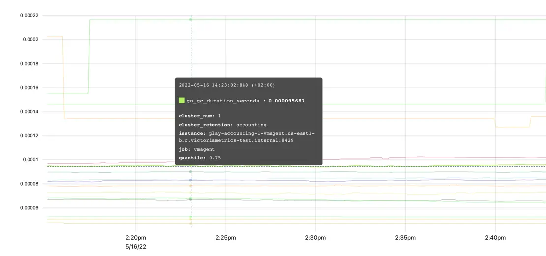
Summary metric type is quite similar to histogram and is used for quantiles calculations. The main difference is that calculations are made on the client-side, so metrics exposition format already contains pre-defined quantiles:
      go_gc_duration_seconds{quantile="0"} 0
go_gc_duration_seconds{quantile="0.25"} 0
go_gc_duration_seconds{quantile="0.5"} 0
go_gc_duration_seconds{quantile="0.75"} 8.0696e-05
go_gc_duration_seconds{quantile="1"} 0.001222168
go_gc_duration_seconds_sum 0.015077078
go_gc_duration_seconds_count 83
The visualization of summaries is pretty straightforward:
Such an approach makes summaries easier to use but also puts significant limitations compared to histograms :
It is impossible to calculate quantile over multiple summary metrics, e.g.
sum(go_gc_duration_seconds{quantile="0.75"}),avg(go_gc_duration_seconds{quantile="0.75"})ormax(go_gc_duration_seconds{quantile="0.75"})won’t return the expected 75th percentile overgo_gc_duration_secondsmetrics collected from multiple instances of the application. See this article for details.It is impossible to calculate quantiles other than the already pre-calculated quantiles.
It is impossible to calculate quantiles for measurements collected over an arbitrary time range. Usually,
summaryquantiles are calculated over a fixed time range such as the last 5 minutes.
Summaries are usually used for tracking the pre-defined percentiles for latency, sizes of elements (batch size, for example) etc.
Instrumenting application with metrics #
As was said at the beginning of the types of metrics section, metric type defines how it was measured. VictoriaMetrics TSDB doesn’t know about metric types. All it sees are metric names, labels, values, and timestamps. What are these metrics, what do they measure, and how - all this depends on the application which emits them.
To instrument your application with metrics compatible with VictoriaMetrics we recommend using github.com/VictoriaMetrics/metrics package. See more details on how to use it in this article .
VictoriaMetrics is also compatible with Prometheus client libraries for metrics instrumentation .
Naming #
We recommend following Prometheus naming convention for metrics . There are no strict restrictions, so any metric name and labels are accepted by VictoriaMetrics. But the convention helps to keep names meaningful, descriptive, and clear to other people. Following convention is a good practice.
Labels #
Every measurement can contain an arbitrary number of key="value" labels. The good practice is to keep this number limited.
Otherwise, it would be difficult to deal with measurements containing a big number of labels.
By default, VictoriaMetrics limits the number of labels per measurement to 40 and drops other labels.
This limit can be changed via -maxLabelsPerTimeseries command-line flag if necessary (but this isn’t recommended).
Every label value can contain an arbitrary string value. The good practice is to use short and meaningful label values to
describe the attribute of the metric, not to tell the story about it. For example, label-value pair
environment="prod" is ok, but log_message="long log message with a lot of details..." is not ok. By default,
VictoriaMetrics limits label’s value size with 4KiB. This limit can be changed via -maxLabelValueLen command-line flag.
It is very important to keep under control the number of unique label values, since every unique label value leads to a new time series . Try to avoid using volatile label values such as session ID or query ID in order to avoid excessive resource usage and database slowdown.
Multi-tenancy #
Cluster version of VictoriaMetrics supports multi-tenancy for data isolation.
Multi-tenancy can be emulated for single-server version of VictoriaMetrics by adding labels on write path and enforcing labels filtering on read path .
Write data #
VictoriaMetrics supports both models used in modern monitoring applications: push and pull .
Push model #
Client regularly sends the collected metrics to the server in the push model:
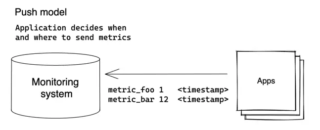
The client (application) decides when and where to send its metrics. VictoriaMetrics supports many protocols
for data ingestion (aka push protocols) - see
the full list here
.
All the protocols are fully compatible with VictoriaMetrics
data model
and can be used in production.
We recommend using the github.com/VictoriaMetrics/metrics
package
for pushing application metrics to VictoriaMetrics.
It is also possible to use already existing clients compatible with the protocols listed above
like Telegraf
for
InfluxDB line protocol
.
Creating custom clients or instrumenting the application for metrics writing is as easy as sending a POST request:
curl -d '{"metric":{"__name__":"foo","job":"node_exporter"},"values":[0,1,2],"timestamps":[1549891472010,1549891487724,1549891503438]}' -X POST 'http://localhost:8428/api/v1/import'
It is allowed to push/write metrics to single-node VictoriaMetrics , to cluster component vminsert and to vmagent .
The pros of push model:
- Simpler configuration at VictoriaMetrics side - there is no need to configure VictoriaMetrics with locations of the monitored applications. There is no need in complex service discovery schemes .
- Simpler security setup - there is no need to set up access from VictoriaMetrics to each monitored application.
See Foiled by the Firewall: A Tale of Transition From Prometheus to VictoriaMetrics elaborating more on why Percona switched from pull to push model.
The cons of push protocol:
- Increased configuration complexity for monitored applications. Every application needs to be individually configured with the address of the monitoring system for metrics delivery. It also needs to be configured with the interval between metric pushes and the strategy in case of metric delivery failure.
- Non-trivial setup for metrics’ delivery into multiple monitoring systems.
- It may be hard to tell whether the application went down or just stopped sending metrics for a different reason.
- Applications can overload the monitoring system by pushing metrics at too short intervals.
Pull model #
Pull model is an approach popularized by Prometheus , where the monitoring system decides when and where to pull metrics from:
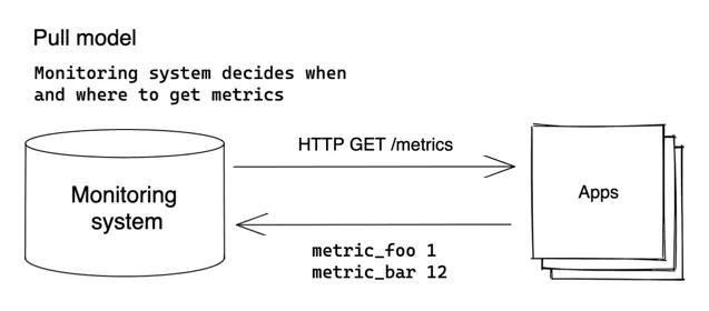
In pull model, the monitoring system needs to be aware of all the applications it needs to monitor. The metrics are
scraped (pulled) from the known applications (aka scrape targets) via HTTP protocol on a regular basis (aka scrape_interval).
VictoriaMetrics supports discovering Prometheus-compatible targets and scraping metrics from them in the same way as Prometheus does - see these docs .
Metrics scraping is supported by single-node VictoriaMetrics and by vmagent .
The pros of the pull model:
- Easier to debug - VictoriaMetrics knows about all the monitored applications (aka
scrape targets). Theup == 0query instantly shows unavailable scrape targets. The actual information about scrape targets is available athttp://victoriametrics:8428/targetsandhttp://vmagent:8429/targets. - Monitoring system controls the frequency of metrics’ scrape, so it is easier to control its load.
- Applications aren’t aware of the monitoring system and don’t need to implement the logic for metrics delivery.
The cons of the pull model:
- Harder security setup - monitoring system needs to have access to applications it monitors.
- Pull model needs non-trivial service discovery schemes .
Common approaches for data collection #
VictoriaMetrics supports both push and pull models for data collection. Many installations use exclusively one of these models, or both at once.
The most common approach for data collection is using both models:
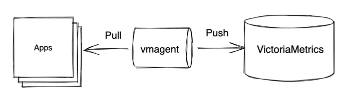
In this approach the additional component is used - vmagent . Vmagent is a lightweight agent whose main purpose is to collect, filter, relabel and deliver metrics to VictoriaMetrics. It supports all push and pull protocols mentioned above.
The basic monitoring setup of VictoriaMetrics and vmagent is described in the example docker-compose manifest . In this example vmagent scrapes a list of targets and forwards collected data to VictoriaMetrics . VictoriaMetrics is then used as a datasource for Grafana installation for querying collected data.
VictoriaMetrics components allow building more advanced topologies. For example, vmagents can push metrics from separate datacenters to the central VictoriaMetrics:
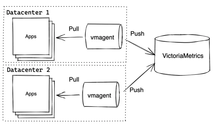
VictoriaMetrics in this example may be either single-node VictoriaMetrics or VictoriaMetrics Cluster . Vmagent also allows replicating the same data to multiple destinations .
Query data #
VictoriaMetrics provides an HTTP API for serving read queries. The API is used in various integrations such as Grafana . The same API is also used by VMUI - a graphical User Interface for querying and visualizing metrics.
The API consists of two main handlers for serving instant queries and range queries .
Instant query #
Instant query executes the query expression at the given time:
GET | POST /api/v1/query?query=...&time=...&step=...&timeout=...
Params:
query- MetricsQL expression.time- optional, timestamp in millisecond precision to evaluate thequeryat. If omitted,timeis set tonow()(current timestamp). Thetimeparam can be specified in multiple allowed formats .step- optional interval for searching for raw samples in the past when executing thequery(used when a sample is missing at the specifiedtime). For example, the request/api/v1/query?query=up&step=1mlooks for the last written raw sample for the metricupin the(now()-1m, now()]interval (the first millisecond is not included). If omitted,stepis set to5m(5 minutes) by default.timeout- optional query timeout. For example,timeout=5s. Query is canceled when the timeout is reached. By default the timeout is set to the value of-search.maxQueryDurationcommand-line flag passed to single-node VictoriaMetrics or tovmselectcomponent of VictoriaMetrics cluster.
The result of Instant query is a list of
time series
matching the filter in query expression. Each returned series contains exactly one (timestamp, value) entry,
where timestamp equals to the time query arg, while the value contains query result at the requested time.
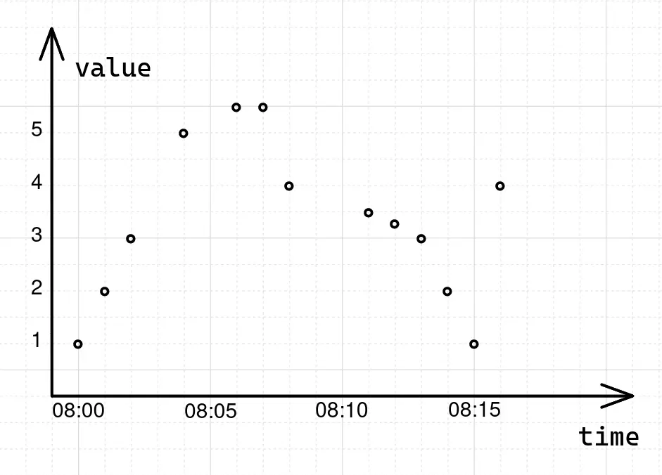
To understand how instant queries work, let’s begin with a data sample:
      foo_bar 1.00 1652169600000 # 2022-05-10T08:00:00Z
foo_bar 2.00 1652169660000 # 2022-05-10T08:01:00Z
foo_bar 3.00 1652169720000 # 2022-05-10T08:02:00Z
foo_bar 5.00 1652169840000 # 2022-05-10T08:04:00Z, one point missed
foo_bar 5.50 1652169960000 # 2022-05-10T08:06:00Z, one point missed
foo_bar 5.50 1652170020000 # 2022-05-10T08:07:00Z
foo_bar 4.00 1652170080000 # 2022-05-10T08:08:00Z
foo_bar 3.50 1652170260000 # 2022-05-10T08:11:00Z, two points missed
foo_bar 3.25 1652170320000 # 2022-05-10T08:12:00Z
foo_bar 3.00 1652170380000 # 2022-05-10T08:13:00Z
foo_bar 2.00 1652170440000 # 2022-05-10T08:14:00Z
foo_bar 1.00 1652170500000 # 2022-05-10T08:15:00Z
foo_bar 4.00 1652170560000 # 2022-05-10T08:16:00Z
The data above contains a list of samples for the foo_bar time series with time intervals between samples
ranging from 1m to 3m. If we plot this data sample on the graph, it will have the following form:
To get the value of the foo_bar series at some specific moment of time, for example 2022-05-10T08:03:00Z, in
VictoriaMetrics we need to issue an instant query:
curl "http://<victoria-metrics-addr>/api/v1/query?query=foo_bar&time=2022-05-10T08:03:00.000Z"
      {
  "status": "success",
  "data": {
    "resultType": "vector",
    "result": [
      {
        "metric": {
          "__name__": "foo_bar"
        },
        "value": [
          1652169780, // 2022-05-10T08:03:00Z
          "3"
        ]
      }
    ]
  }
}
In response, VictoriaMetrics returns a single sample-timestamp pair with a value of 3 for the series
foo_bar at the given moment in time 2022-05-10T08:03:00Z. But, if we take a look at the original data sample again,
we’ll see that there is no raw sample at 2022-05-10T08:03:00Z. When there is no raw sample at the
requested timestamp, VictoriaMetrics will try to locate the closest sample before the requested timestamp:
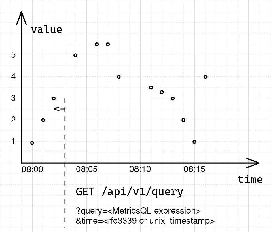
The time range in which VictoriaMetrics will try to locate a replacement for a missing data sample is equal to 5m
by default and can be overridden via the step parameter.
Instant queries can return multiple time series, but always only one data sample per series. Instant queries are used in the following scenarios:
- Getting the last recorded value;
- For
rollup functions
such as
count_over_time; - For alerts and recording rules evaluation;
- Plotting Stat or Table panels in Grafana.
Range query #
Range query executes the query expression at the given [start…end] time range with the given step:
GET | POST /api/v1/query_range?query=...&start=...&end=...&step=...&timeout=...
Params:
query- MetricsQL expression.start- the starting timestamp of the time range forqueryevaluation.end- the ending timestamp of the time range forqueryevaluation. If theendisn’t set, then theendis automatically set to the current time.step- the interval between data points, which must be returned from the range query. Thequeryis executed atstart,start+step,start+2*step, …,start+N*steptimestamps, whereNis the whole number of steps that fit betweenstartandend.endis included only when it equals tostart+N*step. If thestepisn’t set, then it default to5m(5 minutes).timeout- optional query timeout. For example,timeout=5s. Query is canceled when the timeout is reached. By default the timeout is set to the value of-search.maxQueryDurationcommand-line flag passed to single-node VictoriaMetrics or tovmselectcomponent in VictoriaMetrics cluster.
The result of Range query is a list of
time series
matching the filter in query expression. Each returned series contains (timestamp, value) results for the query executed
at start, start+step, start+2*step, …, start+N*step timestamps. In other words, Range query is an
Instant query
executed independently at start, start+step, …, start+N*step timestamps with the only difference that an instant query
does not return ephemeral samples (see below). Instead, if the database does not contain any samples for the requested time and step,
it simply returns an empty result.
For example, to get the values of foo_bar during the time range from 2022-05-10T07:59:00Z to 2022-05-10T08:17:00Z,
we need to issue a range query:
curl "http://<victoria-metrics-addr>/api/v1/query_range?query=foo_bar&step=1m&start=2022-05-10T07:59:00.000Z&end=2022-05-10T08:17:00.000Z"
      {
  "status": "success",
  "data": {
    "resultType": "matrix",
    "result": [
      {
        "metric": {
          "__name__": "foo_bar"
        },
        "values": [
          [
            1652169600,
            "1"
          ],
          [
            1652169660,
            "2"
          ],
          [
            1652169720,
            "3"
          ],
          [
            1652169780,
            "3"
          ],
          [
            1652169840,
            "5"
          ],
          [
            1652169900,
            "5"
          ],
          [
            1652169960,
            "5.5"
          ],
          [
            1652170020,
            "5.5"
          ],
          [
            1652170080,
            "4"
          ],
          [
            1652170140,
            "4"
          ],
          [
            1652170260,
            "3.5"
          ],
          [
            1652170320,
            "3.25"
          ],
          [
            1652170380,
            "3"
          ],
          [
            1652170440,
            "2"
          ],
          [
            1652170500,
            "1"
          ],
          [
            1652170560,
            "4"
          ],
          [
            1652170620,
            "4"
          ]
        ]
      }
    ]
  }
}
In response, VictoriaMetrics returns 17 sample-timestamp pairs for the series foo_bar at the given time range
from 2022-05-10T07:59:00Z to 2022-05-10T08:17:00Z. But, if we take a look at the original data sample again, we’ll
see that it contains only 13 raw samples. What happens here is that the range query is actually
an
instant query
executed 1 + (start-end)/step times on the time range from start to end. If we plot
this request in VictoriaMetrics the graph will be shown as the following:
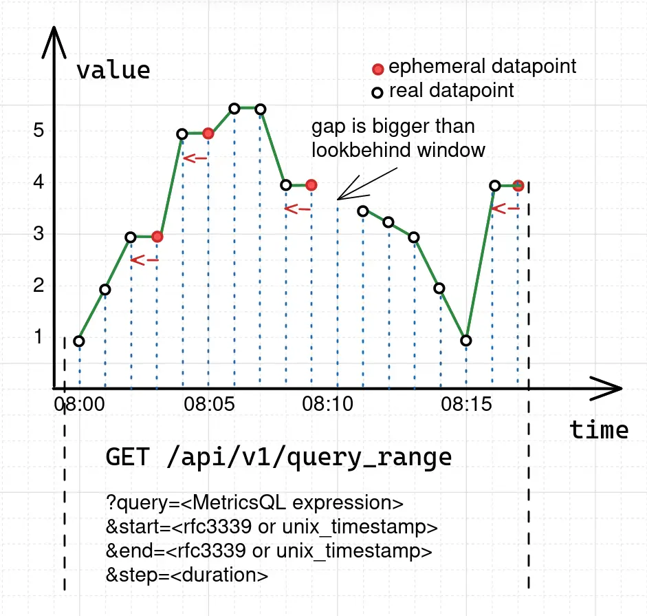
The blue dotted lines in the figure are the moments when the instant query was executed. Since the instant query retains the
ability to return replacements for missing points, the graph contains two types of data points: real and ephemeral.
ephemeral data points always repeat the closest raw sample that occurred before (see red arrow on the pic above).
This behavior of adding ephemeral data points comes from the specifics of the pull model :
- Metrics are scraped at fixed intervals.
- Scrape may be skipped if the monitoring system is overloaded.
- Scrape may fail due to network issues.
According to these specifics, the range query assumes that if there is a missing raw sample then it is likely a missed
scrape, so it fills it with the previous raw sample. The same will work for cases when step is lower than the actual
interval between samples. In fact, if we set step=1s for the same request, we’ll get about 1 thousand data points in
response, where most of them are ephemeral.
Sometimes, the lookbehind window for locating the datapoint isn’t big enough and the graph will contain a gap. For range
queries, lookbehind window isn’t equal to the step parameter. It is calculated as the median of the intervals between
the last 20 raw samples in the requested time range. In this way, VictoriaMetrics automatically adjusts the lookbehind
window to fill gaps and detect stale series at the same time.
Range queries are mostly used for plotting time series data over specified time ranges. These queries are extremely useful in the following scenarios:
- Track the state of a metric on the given time interval;
- Correlate changes between multiple metrics on the time interval;
- Observe trends and dynamics of the metric change.
If you need to export raw samples from VictoriaMetrics, then take a look at export APIs .
Query latency #
By default, Victoria Metrics does not immediately return the recently written samples. Instead, it retrieves the last results
written prior to the time specified by the -search.latencyOffset command-line flag, which has a default offset of 30 seconds.
This is true for both query and query_range and may give the impression that data is written to the VM with a 30-second delay.
This flag prevents from non-consistent results due to the fact that only part of the values are scraped in the last scrape interval.
Here is an illustration of a potential problem when -search.latencyOffset is set to zero:
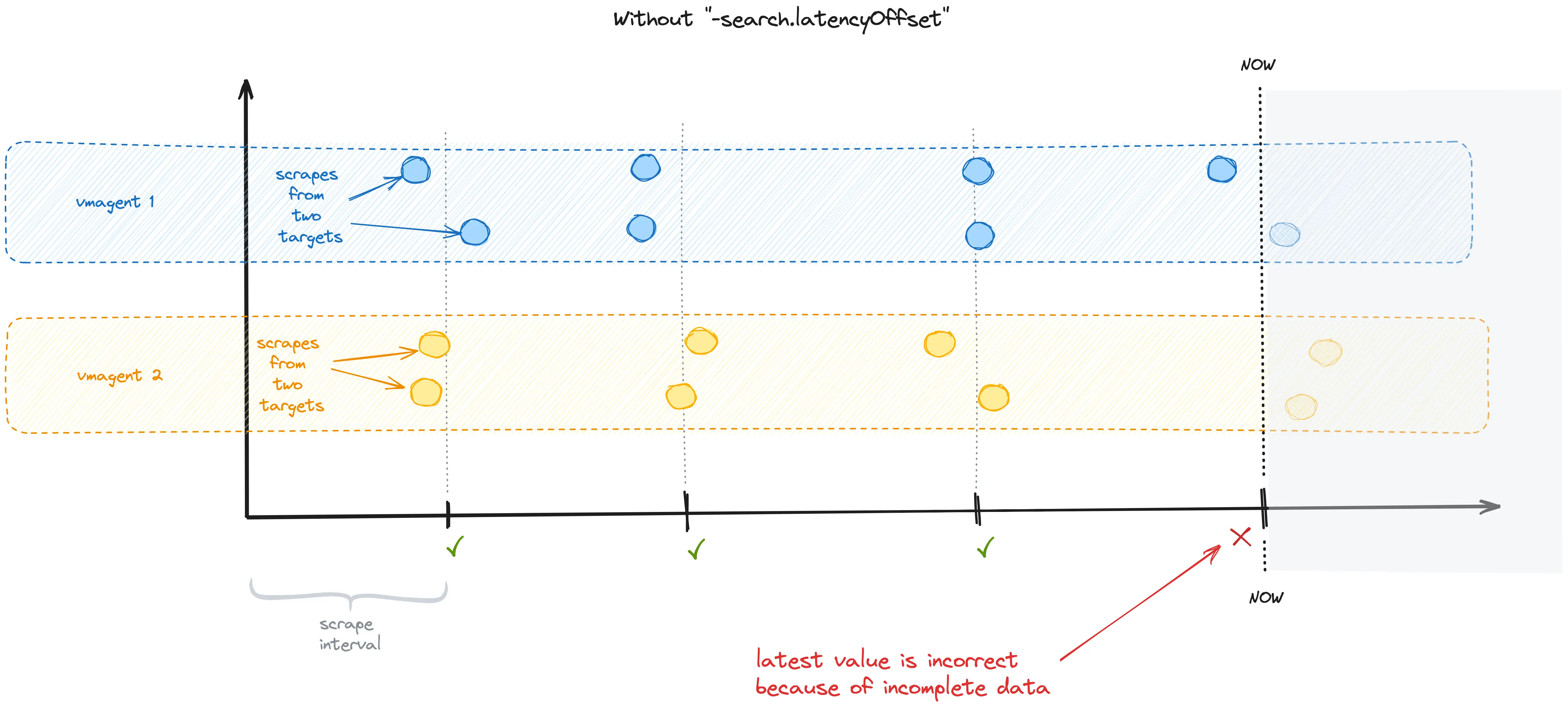
When this flag is set, the VM will return the last metric value collected before the -search.latencyOffset
duration throughout the -search.latencyOffset duration:
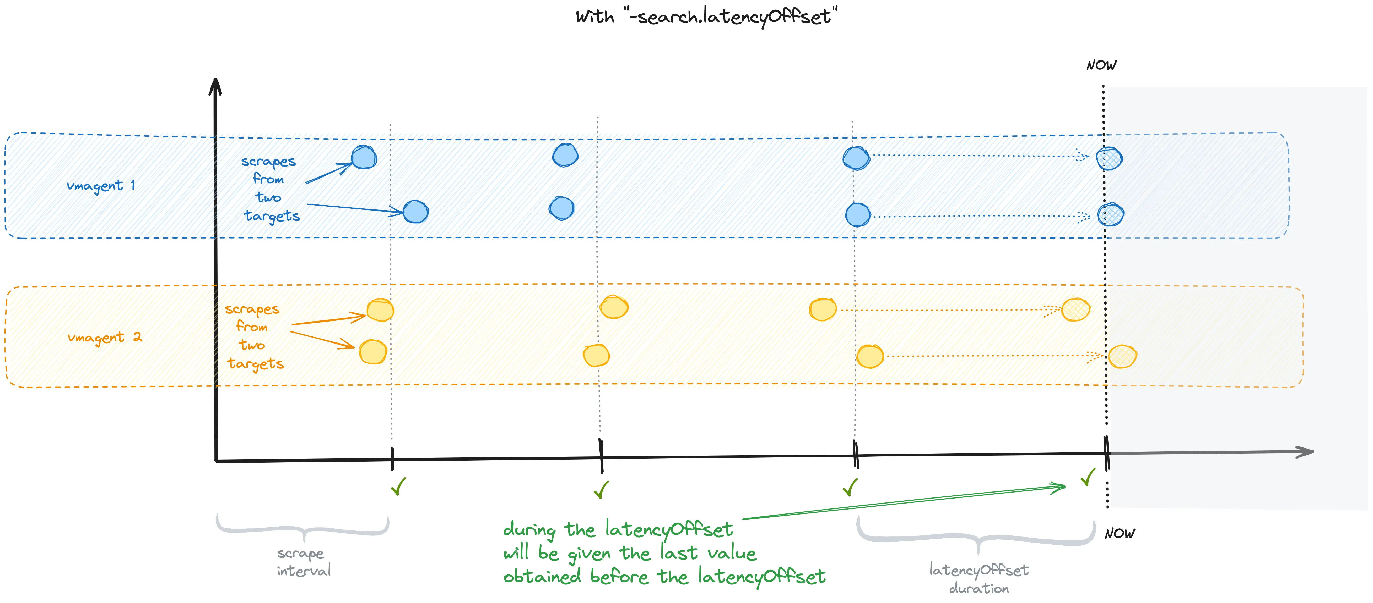
It can be overridden on per-query basis via latency_offset query arg.
VictoriaMetrics buffers recently ingested samples in memory for up to a few seconds and then periodically flushes these samples to disk.
This buffering improves data ingestion performance. The buffered samples are invisible in query results, even if -search.latencyOffset command-line flag is set to 0,
or if latency_offset query arg is set to 0.
You can send GET request to /internal/force_flush http handler at single-node VictoriaMetrics
or to vmstorage at
cluster version of VictoriaMetrics
in order to forcibly flush the buffered samples to disk, so they become visible for querying. The /internal/force_flush handler
is provided for debugging and testing purposes only. Do not call it in production, since this may significantly slow down data ingestion
performance and increase resource usage.
MetricsQL #
VictoriaMetrics provide a special query language for executing read queries - MetricsQL . It is a PromQL -like query language with a powerful set of functions and features for working specifically with time series data. MetricsQL is backward-compatible with PromQL, so it shares most of the query concepts. The basic concepts for PromQL and MetricsQL are described here .
Filtering #
In sections
instant query
and
range query
we’ve already used MetricsQL to get data for
metric foo_bar. It is as simple as just writing a metric name in the query:
foo_bar
A single metric name may correspond to multiple time series with distinct label sets. For example:
      requests_total{path="/", code="200"}
requests_total{path="/", code="403"}
To select only time series with specific label value specify the matching filter in curly braces:
requests_total{code="200"}
The query above returns all time series with the name requests_total and label code="200". We use the operator = to
match label value. For negative match use != operator. Filters also support positive regex matching via =~
and negative regex matching via !~:
requests_total{code=~"2.*"}
Filters can also be combined:
requests_total{code=~"200", path="/home"}
The query above returns all time series with requests_total name, which simultaneously have labels code="200" and path="/home".
Filtering by name #
Sometimes it is required to return all the time series for multiple metric names. As was mentioned in
the
data model section
, the metric name is just an ordinary label with a special name - __name__. So
filtering by multiple metric names may be performed by applying regexps on metric names:
{__name__=~"requests_(error|success)_total"}
The query above returns series for two metrics: requests_error_total and requests_success_total.
Filtering by multiple “or” filters #
MetricsQL
supports selecting time series, which match at least one of multiple “or” filters.
Such filters must be delimited by or inside curly braces. For example, the following query selects time series with
{job="app1",env="prod"} or {job="app2",env="dev"} labels:
{job="app1",env="prod" or job="app2",env="dev"}
The number of or groups can be arbitrary. The number of ,-delimited label filters per each or group can be arbitrary.
Per-group filters are applied with and operation, e.g. they select series simultaneously matching all the filters in the group.
This functionality allows passing the selected series to rollup functions such as rate() without the need to use subqueries :
rate({job="app1",env="prod" or job="app2",env="dev"}[5m])
If you need to select series matching multiple filters for the same label, then it is better from performance PoV
to use regexp filter {label=~"value1|...|valueN"} instead of {label="value1" or ... or label="valueN"}.
Arithmetic operations #
MetricsQL supports all the basic arithmetic operations:
- addition -
+ - subtraction -
- - multiplication -
* - division -
/ - modulo -
% - power -
^
This allows performing various calculations across multiple metrics. For example, the following query calculates the percentage of error requests:
(requests_error_total / (requests_error_total + requests_success_total)) * 100
Combining multiple series #
Combining multiple time series with arithmetic operations requires an understanding of matching rules. Otherwise, the query may break or may lead to incorrect results. The basics of the matching rules are simple:
- MetricsQL engine strips metric names from all the time series on the left and right side of the arithmetic operation without touching labels.
- For each time series on the left side MetricsQL engine searches for the corresponding time series on the right side with the same set of labels, applies the operation for each data point and returns the resulting time series with the same set of labels. If there are no matches, then the time series is dropped from the result.
- The matching rules may be augmented with
ignoring,on,group_leftandgroup_rightmodifiers. See these docs for details.
Comparison operations #
MetricsQL supports the following comparison operators:
- equal -
== - not equal -
!= - greater -
> - greater-or-equal -
>= - less -
< - less-or-equal -
<=
These operators may be applied to arbitrary MetricsQL expressions as with arithmetic operators. The result of the
comparison operation is time series with only matching data points. For instance, the following query would return
series only for processes where memory usage exceeds 100MB:
process_resident_memory_bytes > 100*1024*1024
Aggregation and grouping functions #
MetricsQL allows aggregating and grouping of time series. Time series are grouped by the given set of labels and then the
given aggregation function is applied individually per each group. For instance, the following query returns
summary memory usage for each job:
sum(process_resident_memory_bytes) by (job)
See docs for aggregate functions in MetricsQL .
Calculating rates #
One of the most widely used functions for
counters
is
rate
. It calculates the average per-second increase rate individually
per each matching time series. For example, the following query shows the average per-second data receive speed
per each monitored node_exporter instance, which exposes the node_network_receive_bytes_total metric:
rate(node_network_receive_bytes_total)
By default, VictoriaMetrics calculates the rate over
raw samples
on the lookbehind window specified in the step param
passed either to
instant query
or to
range query
.
The interval on which rate needs to be calculated can be specified explicitly
as duration
in square brackets:
rate(node_network_receive_bytes_total[5m])
In this case VictoriaMetrics uses the specified lookbehind window - 5m (5 minutes) - for calculating the average per-second increase rate.
Bigger lookbehind windows usually lead to smoother graphs.
rate strips metric name while leaving all the labels for the inner time series. If you need to keep the metric name,
then add
keep_metric_names
modifier
after the rate(..). For example, the following query leaves metric names after calculating the rate():
rate(node_network_receive_bytes_total) keep_metric_names
rate() must be applied only to
counters
. The result of applying the rate() to
gauge
is undefined.
Visualizing time series #
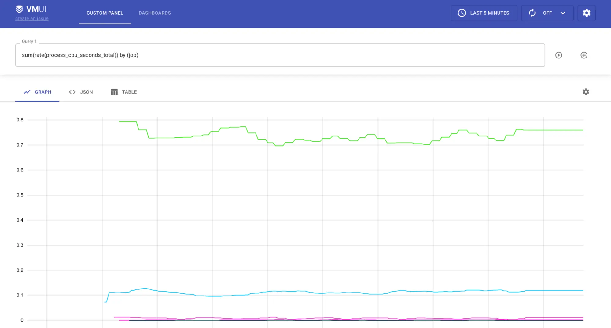
VictoriaMetrics has a built-in graphical User Interface for querying and visualizing metrics -
VMUI
.
Open http://victoriametrics:8428/vmui page, type the query and see the results:
VictoriaMetrics supports Prometheus HTTP API which makes it possible to query it with Grafana in the same way as Grafana queries Prometheus.
Modify data #
VictoriaMetrics stores time series data in MergeTree -like data structures. While this approach is very efficient for write-heavy databases, it applies some limitations on data updates. In short, modifying already written time series requires re-writing the whole data block where it is stored. Due to this limitation, VictoriaMetrics does not support direct data modification.
Deletion #
See How to delete time series .
Relabeling #
Relabeling is a powerful mechanism for modifying time series before they have been written to the database. Relabeling may be applied for both push and pull models. See more details here .
Deduplication #
VictoriaMetrics supports data deduplication. See these docs .
Downsampling #
VictoriaMetrics supports data downsampling. See these docs .